Chapter 6 Mapping and Spatial Analysis

This chapter was contributed by Henry Hershey

6.1 Chapter Overview

R is a relatively under-used tool for creating Geographic Information Systems (GIS). Most people use ArcGIS, QGIS, or Google Earth to display and analyze spatial data. However, R can do much of what you might want to do in those programs, with the added benefit of allowing you to create a reproducible script file to share. Workflows can be difficult to replicate in ArcGIS because of the point-click user interface. With R, anyone can replicate your geospatial analysis with your script file and data.

In this chapter, you will learn the basics of:

• creating a GIS in R
• mapping parts of your GIS
• “selecting by attribute” (A.K.A.subset() or dplyr::filter() in R)
• manipulating spatial objects

You will map and analyze data from a brown bear (Ursus arctos) tracking study (Kaczensky et al. 1999). In Slovenia, a railroad connects the capitol Ljubljana with the coastal city of Koper, and passes right through brown bear country. You will use R to assess potential sites to build a hypothetical wildlife overpass so that bears can safely cross the railroad.

It is worth mentioning that if you are left wanting more information about geospatial analysis in R after this brief introduction, a thorough description of more advanced techniques is presented for free in Lovelace, Nowosad, and Muenchow (2018).

6.2 Before You Begin

You should create a new directory and R script for your work in this chapter called Ch6.R and save it in the directory C:/Users/YOU/Documents/R-Book/Chapter6. Set your working directory to that location. Revisit the material in Sections 1.2 and 1.3 for more details on these steps.

For this chapter, it will be helpful to have the data in your working directory. In the Data/Ch6 folder (see the instructions on acquiring the data files), you’ll find:

1. a file named bear.csv,
2. folders named railways, states, and SVN_adm, and
3. an R script called points_to_line.R (Walker 2015).

Copy (or cut if you’d like) all of these files/folders from Data/Ch6 into your working directory.

Mapping in R requires many packages. Install all of the following packages:

install.packages(
  c("sp","rgdal","maptools",
  "rgeos","raster","scales",
  "adehabitatHR","dismo", "prettymapr")
)

You will need {dplyr} (Wickham et al. 2017) as well, if you did not install it already for Chapter 5.

Rather than load all the packages at the top of the script (as is typically customary), this chapter will load and briefly describe each package immediately prior to using it for the first time.

6.3 Geospatial Data

There are two types of geospatial data: vector⁴³ and raster data. R is able to handle both, but for the sake of simplicity, this chapter will mostly deal with vector data. There are three types of vector data that you should be familiar with (Figure 6.1):

• A point is a pair of coordinates (x = longitude, y = latitude) that represent the location of some observed object or event
• A line is a path between two or more ordered points. The endpoints of a line are called vertices.
• A polygon is an area bounded by vertices that are connected in order. In a polygon, the first and last vertex are the same.

In this first section, you will learn how to load these different types of data and create spatial objects that you can manipulate and visualize in R.

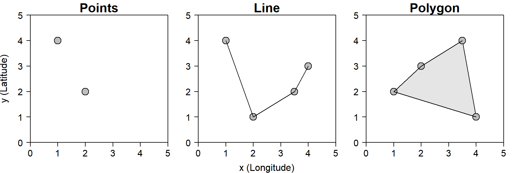
Figure 6.1: The three basic types of GIS vector data

6.4 Importing Geospatial Data

6.4.1 .csv files

Begin by loading in coordinate data from bear.csv and creating a points layer from them. The points are from a telemetry study that tracked brown bear movements in south western Slovenia for a period of about 10 years (Kaczensky et al. 1999). Each observation in this data set represents what is called a relocation event - meaning a bear was detected again after it was initially tagged. The variables measured at each relocation event include a location, a time, and several other variables.

bear = read.csv("bear.csv",stringsAsFactors = F)
colnames(bear)

##  [1] "event.id"                        "visible"                        
##  [3] "timestamp"                       "location.long"                  
##  [5] "location.lat"                    "behavioural.classification"     
##  [7] "comments"                        "location.error.text"            
##  [9] "sensor.type"                     "individual.taxon.canonical.name"
## [11] "tag.local.identifier"            "individual.local.identifier"    
## [13] "study.name"                      "utm.easting"                    
## [15] "utm.northing"                    "utm.zone"

There are quite a few variables in these data that are extraneous, so just keep the bare necessities: the date and time a bear was relocated, the name of the observed bear, and the x and y coordinates of its relocation. Also, omit the observations that have an NA value for any of those variables with na.omit():

bear = na.omit(bear[,c("timestamp","tag.local.identifier",
                        "location.long","location.lat")])
colnames(bear) = c("timestamp","ID","x","y")
head(bear)

##             timestamp    ID        x        y
## 1 1994-04-23 22-00-00 ancka 14.32837 45.88914
## 2 1994-04-24 16-40-00 ancka 14.37175 45.87072
## 3 1994-04-25 14-45-00 ancka 14.39852 45.86659
## 4 1994-04-26 12-30-00 ancka 14.41215 45.88695
## 5 1994-04-28 12-00-00 ancka 14.41260 45.87476
## 6 1994-04-29 09-30-00 ancka 14.40471 45.88957

Notice that the bears have names: unique(bear$ID). Do some more simple data wrangling:

# how many records of each bear are there?
table(bear$ID)

## 
##  ancka   clio  dinko  dusan   ivan   jana  janko   joze   jure klemen 
##    351     20     11     43      7    111      7     24     17     19 
##  lucia   maja  metka  milan mishko   nejc polona srecko  urosh  vanja 
##    169    247     66      3    129    117    208    138     21     65 
##   vera  vinko 
##     92     33

# bears that were relocated fewer than 5 times 
# cannot be used in future analysis so filter them out
library(dplyr)
bear = bear %>%
  group_by(ID) %>%
  filter(n() >= 5)

# now how many bears are there?
unique(bear$ID)

##  [1] "ancka"  "clio"   "dinko"  "dusan"  "ivan"   "jana"   "janko" 
##  [8] "joze"   "jure"   "klemen" "lucia"  "maja"   "metka"  "mishko"
## [15] "nejc"   "polona" "srecko" "urosh"  "vanja"  "vera"   "vinko"

Now, use the {sp} package (Pebesma and Bivand 2018) to create a spatial object out of your standard R data frame. You can think of this object like a layer in GIS. {sp} lets you create layers with or without attribute tables, but if your spatial data have other attributes like an ID or a timestamp variable, you should always create an object with class SpatialPointsDataFrame to make sure those variables/attributes are stored.

In order to convert a data frame into a SpatialPointsDataFrame, you need to specify four arguments:

• data: the data frame being converted,
• coords: the coordinates in that dataframe,
• coords.nrs: the indices for those coordinate vectors in the data data.frame, and
• proj4string: the projected coordinate system of the data. You will use the WGS84 coordinate reference system. More on coordinate reference systems later in Section 6.6.1⁴⁴.

library(sp)
bear = SpatialPointsDataFrame(
  data = bear,
  coords = bear[,c("x","y")],
  coords.nrs = c(3,4),
  proj4string = CRS("+init=epsg:4326")
  )

Without any reference data these points are essentially useless. You will need to load some more spatial data to get your bearings. You have more spatial data, but they are in a different format.

6.4.2 .shp files

The {rgdal} package (Bivand, Keitt, and Rowlingson 2018) facilitates loading spatial data files (i.e., shapefiles) into R. The function readOGR() takes a standard shapefile (.shp), and converts it into a spatial object of the appropriate class (e.g., points or polygons). It takes two arguments: the data source name (dsn, the directory), and the layer name (layer). When you download a shapefile from an open-source web portal, it will often have accompanying files that store the attribute data. Store all of these files in a folder with the same name as the shapefile. Now load in the shapefile that contains a polygon for the boundary of Slovenia (Boundaries 2018) from the directory, so you can see where in the country the brown bears were detected:

#load all the shapefiles for the background map. 
#you'll learn how to add a basemap later
library(rgdal)
#border of slovenia
slovenia = readOGR(dsn = "./SVN_adm",layer = "SVN_adm0")

There are two important differences between readOGR() and read.csv():

1. The directory shortening syntax is not the same. Notice the period in the data source names. This indicates your working directory.
2. When calling the layer name, the file extension .shp is not required.

Notice the feature class of slovenia is a polygon:

class(slovenia)

## [1] "SpatialPolygonsDataFrame"
## attr(,"package")
## [1] "sp"

Now read in two other shapefiles:

• one showing the statistical regions (aka states) of Slovenia (Boundaries 2018)
• one showing the railways in Slovenia (MapCruzin 2018)

#major railroads in slovenia
railways = readOGR(dsn = "./railways",
                   layer = "railways") 
#statistical areas (states)
stats = readOGR(dsn = "./SVN_adm",
                layer = "SVN_adm1", stringsAsFactors = F)  

6.5 Plotting

Plotting spatial objects in R is a breeze. See what happens if you just plot the bear object:

plot(bear)

You can clean up your map a bit with standard {graphics} arguments:

library(scales)
par(mar = c(2,2,1,1))
plot(bear, col = alpha("blue", 0.5), pch = 16, axes = T)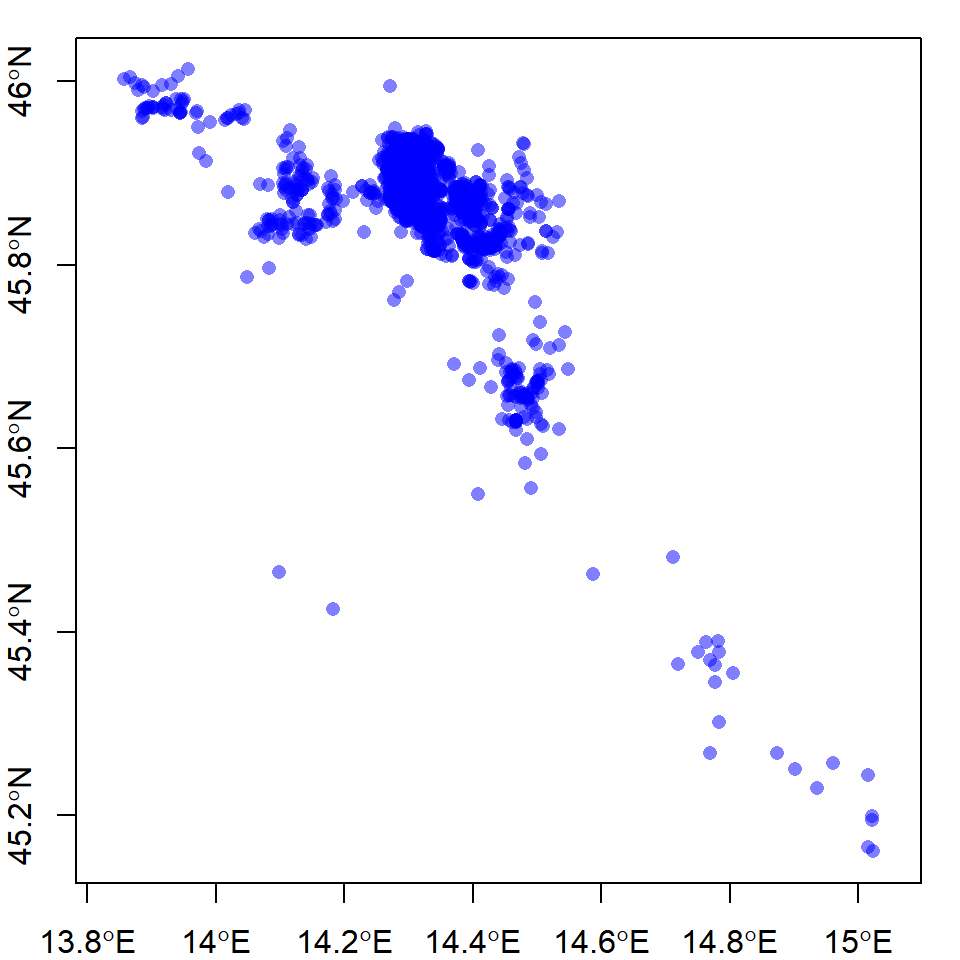

The alpha() function from the {scales} package (Wickham 2018) allows you to plot with transparent colors, which is helpful for seeing the high- versus low-density clusters. Now, plot your reference layers to get your bearings:

#make a map of all the bear relocations and railways in slovenia
par(mar = c(2,2,1,1))
plot(stats, border = "grey", axes = T)
plot(slovenia, lwd = 3, add = T)     # you can draw multiple plots on top
points(bear, pch = 16, cex = 0.5,    # or use a low lvl plot function
       col = alpha("blue", 0.5))
lines(railways, col = "red", lwd = 3) 

6.5.1 Zooming

You may want to zoom in on the part of Slovenia where the bears are. Spatial objects in R have a slot⁴⁵ called bbox which is the “boundary box” of the data in that object. You can use the bbox to specify what the xlim and ylim of your map should be:

plot(stats, border = "grey", axes = T,
     xlim = bear@bbox[1,],  # access the boundary box using @
     ylim = bear@bbox[2,])
plot(slovenia, lwd = 3, add = T)
points(bear, pch = 16, cex = 0.5, col = alpha("blue", 0.5))
plot(railways, add = T, col = "red", lwd = 3)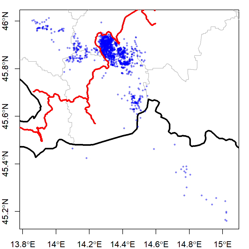

6.5.2 Plotting Selections

In GIS, a subset is often called a selection; it is a smaller subset of a larger data layer. Say you want to see the relocation events for each individual bear at a time. Use sapply() to apply a function to plot each bear’s track on a separate map. Wrap your code inside of a new PDF device (described in Section 2.10.2) so you can scroll through the plots separately:

pdf("Relocations.pdf", h = 5, w = 5)
sapply(unique(bear$ID), function(id) {
  par(mar = c(2,2,1,1))
  plot(stats, border = "grey", axes = T,
       xlim = bear@bbox[1,],  # access the boundary box using @
       ylim = bear@bbox[2,], main = paste("Bear:", id))
  plot(slovenia, lwd = 3, add = T)
  points(bear[bear$ID == id,], type = "o", pch = 16, cex = 0.5, col = alpha("blue", 0.5))
  plot(railways, add = T, col = "red", lwd = 3)
})
dev.off()

When you run this code, it will look like nothing happened. Go to your working directory and open the newly created file Relocations.pdf to see the output. Note that if you want to make changes to the PDF file by running pdf(...); plot(...); dev.off(), you’ll need to close the file in your PDF viewer beforehand⁴⁶.

6.6 Manipulating Spatial Data

Now that you have some data and you’ve taken a look at it, it’s time to learn a few tricks for manipulating them. Looking at your map, see that some of the bears were detected outside of Slovenia. (Bonus points if you can name the country they’re in). Suppose the Slovenian government can’t build wildlife crossings in other countries, so you have to clip the bear data to the boundary of Slovenia.

6.6.1 Changing the CRS

Before you can manipulate any two related layers (e.g., clipping), you have to ensure that the two layers have identical coordinate systems. This can be done easily with the spTransform() function in the {sp} package. In order to obtain the coordinate reference system of a spatial object like bear, all you have to do is call proj4string(bear). You can pass this directly to spTransform() like this:

slovenia = spTransform(slovenia, CRS(proj4string(bear))) 

6.6.2 Clipping

Clipping is as simple as a standard subset in R. You can select the relocations that occured only in Slovenia using:

bear = bear[slovenia,]

Make the same plot as you did in Section 6.5.1 with the clipped bear points.

6.6.3 Adding Attributes

What if you wanted to add an attribute to a points object, like the name of the polygon it occurs in? You can find this by extracting the attribute values of one layer (a target) at locations of another layer (a source) with the over() function from the {sp} package. For example, say you wanted to know what statistical region each bear relocation happened in. In this case, the target is the stats layer, and the source is bear layer. These two layers will need to be in the same projection, and the result will be stored in the column bearstats$NAME_1:

# get in same projection
stats = spTransform(stats, proj4string(bear))
# determine which polygon of stat each bear relocation occured in
bearstats = over(bear,stats)
head(bearstats)

##   ID_0 ISO   NAME_0 ID_1             NAME_1             TYPE_1
## 1  208 SVN Slovenia    7  Osrednjeslovenska Statisticna Regije
## 2  208 SVN Slovenia    7  Osrednjeslovenska Statisticna Regije
## 3  208 SVN Slovenia    5 Notranjsko-kraška Statisticna Regije
## 4  208 SVN Slovenia    7  Osrednjeslovenska Statisticna Regije
## 5  208 SVN Slovenia    7  Osrednjeslovenska Statisticna Regije
## 6  208 SVN Slovenia    7  Osrednjeslovenska Statisticna Regije
##            ENGTYPE_1 NL_NAME_1        VARNAME_1
## 1 Statistical Region      <NA>        Ljubljana
## 2 Statistical Region      <NA>        Ljubljana
## 3 Statistical Region      <NA> Kraška, Notranj
## 4 Statistical Region      <NA>        Ljubljana
## 5 Statistical Region      <NA>        Ljubljana
## 6 Statistical Region      <NA>        Ljubljana

Extract just the column you care about and see how many relocations occurred in each state:

bearstats = data.frame(stat = bearstats$NAME_1)
table(bearstats$stat) 

## 
##              Goriška Jugovzhodna Slovenija    Notranjsko-kraška 
##                    65                     2                   823 
##     Osrednjeslovenska 
##                   978

Then, you can recombine your extracted attribute values (in bearstats) to your original layer (bear) with spCbind() from the {maptools} package (Bivand and Lewin-Koh 2018):

library(maptools)
bear = spCbind(bear, bearstats$stat)
head(bear@data)

##             timestamp    ID        x        y     bearstats.stat
## 1 1994-04-23 22-00-00 ancka 14.32837 45.88914  Osrednjeslovenska
## 2 1994-04-24 16-40-00 ancka 14.37175 45.87072  Osrednjeslovenska
## 3 1994-04-25 14-45-00 ancka 14.39852 45.86659 Notranjsko-kraška
## 4 1994-04-26 12-30-00 ancka 14.41215 45.88695  Osrednjeslovenska
## 5 1994-04-28 12-00-00 ancka 14.41260 45.87476  Osrednjeslovenska
## 6 1994-04-29 09-30-00 ancka 14.40471 45.88957  Osrednjeslovenska

Now determine how many times each bear was relocated in each state:

table(bear$ID, bear$bearstats.stat)

6.7 Analysis

Now that you know how to import, plot, and manipulate your data, it’s time to do some analysis. The {rgeos} package (Bivand and Rundel 2018) has a few tools for simple geometric calculations like finding the distance between two points, or the area of a polygon. However, more specialized analyses are often only available in other packages. Two common analytical tasks in animial tracking are:

• Calculating the home range of an animal, i.e., defining the area where most of the relocations occurred.
• Finding intersections between tracks and some other line (e.g., river, state boundary, or railroad).

In this section, you will use the {rgeos} package and another specialized package to do these tasks.

6.7.1 Home Range Analysis

If you look at the plots in Section 6.5.2, it looks like some bears live very close to the railroad, but do not cross it, some live very far away, and others may have crossed it multiple times. Which bears’ home ranges are intersected by the railroad? In order to determine this, you will have to calculate the home range of each animal with the mcp function in the {adehabitatHR} package (Calenge 2006).

library(adehabitatHR) 
#the mcp function requires coordinates 
#be in the Universal Transverse Mercator system
bear = spTransform(bear,CRS("+proj=utm +north +zone=33 +ellps=WGS84"))
# calculate the home range. mcp is one of 5 functions to do this
cp = mcp(xy=bear[,2], percent=95,unin="m",unout="km2") 

mcp calculates the minimum convex polygon bounded by the extent of the points which are within some percentile of closeness to the centroid of a group. Points that are very far away from the center are excluded. The standard percentile is 95%. mcp requires three other arguments:

• xy: the grouping variable of the spatial points data frame (the ID of each bear),
• unin: the units of the input (meters is the default), and
• unout: the units of the output.

If you run cp, you’ll see that the areas of each polygon are stored in the object in square kilometers.

Now, plot the homeranges of each bear, label them using the {rgeos} package, and overlay the railroad on a map.

library(rgeos) 
#match the coordinate system of the home ranges object with the railways layer 
cp = spTransform(cp, CRS(proj4string(slovenia)))
railways = spTransform(railways, CRS(proj4string(slovenia)))
#keep only the homeranges that include some part of the railway
cp = cp[railways,] 

# plot the polygons
par(mar = c(2,2,1,1))
plot(cp,col=alpha("blue", 0.5), axes = T)
#rgeos has a bunch of neat functions like this one
polygonsLabel(cp, labels = cp$id, method = "buffer",
              col = "white", doPlot=T) 
lines(railways, lwd = 3,col = "red")

6.7.2 Finding Intersections Between Two Layers

Now that you know which bears crossed the railroad, find out where. You’ll need a user-defined function called points_to_line(), which is stored as a script file in your working directory (Walker 2015). If you ever write a function, you can store it in a script file, and then bring it into your current session using the source() function. This prevents you from needing to paste all the function code every time you want to use it in a new script. Save as many functions as you want in a single script, and they will all be added to your Global Environment when you source() the file⁴⁷.

source("points_to_line.R")

source("Data/Ch6/points_to_line.R")

source() essentially highlights all the code in a script and runs it, without you ever having to open the script.

# {maptools} is needed by points_to_line()
library(maptools) 
# change CRS
bear = spTransform(bear, CRS(proj4string(slovenia)))
#turn the bear relocations into tracks
bearlines = points_to_line(
  as.data.frame(bear),
  long="x",lat="y",
  id_field="ID", sort_field = "timestamp")

Now that your points have been turned into tracks for each bear, see where they intersect the railroad using the gIntersection() function from the {rgeos} package. Hang on though, this will take your computer a while to run (between 5 and 20 minutes). Optionally, you can start a timer and have the {beepr} package (Bååth 2018) make a sound when the geoprocessing calculations are completed:

library(beepr)
start = Sys.time()
crossings = gIntersection(bearlines, railways) 
Sys.time() - start; beep(10)

6.8 Creating a Presentable Map

Now that you have a points object with the crossings stored, make a map that you can present to policy makers.

First, you should get a nicer basemap than R’s blank slate. Use the {dismo} (Hijmans et al. 2017) and {raster} (Hijmans 2017) packages to get one:

library(dismo); library(raster)
base = gmap(bear, type = "terrain", lonlat = T)
plot(base)

Now, put the rest of the layers in the same projection as the basemap:

# put the other layers in the same crs as the basemap
bear = spTransform(bear, basemap@crs) #note that the method for getting the crs is different for raster objects
railways = spTransform(railways, base@crs)
slovenia = spTransform(slovenia, base@crs)
proj4string(crossings) = base@crs

Now, plot the crossings in blue on top of the basemap with the railroad in red. You can add a scale bar and north arrow using the {prettymapr} (Dunnington 2017) package!

# plot the basemap
plot(base)

# draw on the railways and crossing events
lines(railways, lwd = 10, col = "red")
points(crossings, col = alpha("blue", 0.5), cex = 5, pch = 16)

# draw on a legend
legend("bottom", legend = c("Railway", "Crossing Events"),
       lty = c(1,NA), col = c("red", alpha("blue", 0.5)),
       pch = c(NA, 16), lwd = 10, cex = 5, horiz = T, bty = "n")

# draw on other map components: scale bar and north arrow
look at maptools
addscalebar(plotunit = "latlon", htin = 0.5,
            label.cex = 5, padin = c(0.5,0.5))
addnortharrow(pos = "topleft", scale = 5, padin = c(2, 2.5))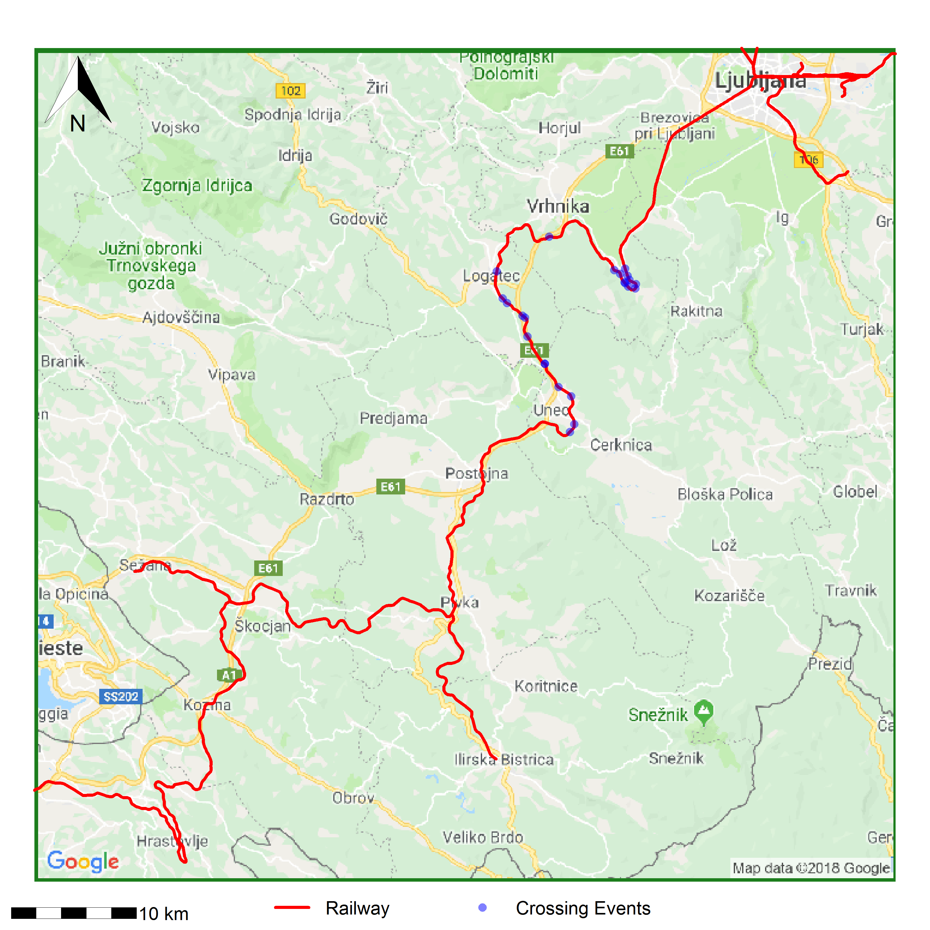

Where are the bears crossing the railroad? It looks like there are two areas of the railroad that get the most bear activity. One in the hairpin turn, and one that’s more spread out between Logatec and Unec. Perhaps there should be wildlife crossings in those areas to protect the more “adventurous” bears.

6.9 Other R Mapping Packages

This chapter has covered many of R’s basic mapping capabilities using the built-in plot() functionality, but there are certainly other frameworks in R. Here are a few examples, and a quick Google search should provide you with plenty of information to get up and running.

6.9.1 {ggmap}

Just like for {ggplot2} (Wickham and Chang 2016), many R users find the {ggmap} (Kahle and Wickham 2016) package more intuitive than creating maps with plot() like you have done in this chapter. If you have messed around with {ggplot2} or would like a slightly different plotting workflow, look into it more.

6.9.2 {leaflet}

The {leaflet} package (Cheng, Karambelkar, and Xie 2018) allows you to make interactive maps. This will only work if your output is HTML-based⁴⁸

library(leaflet)
leaflet() %>%
  #add a basemap
  addProviderTiles(providers$Esri.WorldGrayCanvas, group = "Grey") %>%
  # change the initial zoom
  fitBounds(slovenia@bbox["x","min"], slovenia@bbox["y","min"],
            slovenia@bbox["x","max"], slovenia@bbox["y","max"]) %>%
  # fill in slovenia
  addPolygons(data = slovenia, color = "grey") %>%
  # draw the railroad
  addPolylines(data = railways,opacity = 1, color = "red") %>%
  # draw the relocations
  addCircleMarkers(data = bear, color = "blue", clusterOptions = markerClusterOptions()) %>%
  # draw the crossing events
  addCircleMarkers(data = crossings, color = "yellow", clusterOptions = markerClusterOptions())

Exercise 6

1. Load the caves.shp shapefile (Republic of Slovenia 2018) from your working directory. Add the data to one of the maps of Slovenia you created in this chapter.
2. How many caves are there?
3. How many caves are in each statistical area?
4. Which bear has the most caves in its homerange?

Exercise 6 Bonus

1. Find some data online for a system you are interested in and do similar activities as shown in this chapter. Good examples for obtaining open access spatial data are:

• Administrative boundaries: https://gadm.org/
• Animal tracking data sets: https://www.movebank.org/
• US Geological Survey: https://www.usgs.gov/products/maps/gis-data

References

Bååth, Rasmus. 2018. Beepr: Easily Play Notification Sounds on Any Platform. https://CRAN.R-project.org/package=beepr.

Bivand, Roger, Tim Keitt, and Barry Rowlingson. 2018. Rgdal: Bindings for the ’Geospatial’ Data Abstraction Library. https://CRAN.R-project.org/package=rgdal.

Bivand, Roger, and Nicholas Lewin-Koh. 2018. Maptools: Tools for Handling Spatial Objects. https://CRAN.R-project.org/package=maptools.

Bivand, Roger, and Colin Rundel. 2018. Rgeos: Interface to Geometry Engine - Open Source (’Geos’). https://CRAN.R-project.org/package=rgeos.

Boundaries, Global Administrative. 2018. “Slovenia Geopackage.” https://biogeo.ucdavis.edu/data/gadm3.6/gpkg/gadm36_SVN_gpkg.zip.

Calenge, C. 2006. “The Package Adehabitat for the R Software: Tool for the Analysis of Space and Habitat Use by Animals.” Ecological Modelling 197: 1035.

Cheng, Joe, Bhaskar Karambelkar, and Yihui Xie. 2018. Leaflet: Create Interactive Web Maps with the Javascript ’Leaflet’ Library. https://CRAN.R-project.org/package=leaflet.

Dunnington, Dewey. 2017. Prettymapr: Scale Bar, North Arrow, and Pretty Margins in R. https://CRAN.R-project.org/package=prettymapr.

Hijmans, Robert J. 2017. Raster: Geographic Data Analysis and Modeling. https://CRAN.R-project.org/package=raster.

Hijmans, Robert J., Steven Phillips, John Leathwick, and Jane Elith. 2017. Dismo: Species Distribution Modeling. https://CRAN.R-project.org/package=dismo.

Kaczensky, P., F. Knauer, M. Jonozovic, and M. Blazic. 1999. “Slovenian Brown Bear 1993-1999 Telemetry Data Set.” https://www.movebank.org/panel_embedded_movebank_webapp?destination=panel_embedded_movebank_webapp.

Kahle, David, and Hadley Wickham. 2016. Ggmap: Spatial Visualization with Ggplot2. https://CRAN.R-project.org/package=ggmap.

Lovelace, R., J. Nowosad, and J. Muenchow. 2018. Geocomputation with R. 1st ed. Boca Raton, Florida: Chapman; Hall/CRC. https://geocompr.robinlovelace.net/.

MapCruzin. 2018. “Slovenia Railways.” http://www.mapcruzin.com/download-shapefile/slovenia-railways-shape.zip.

Pebesma, Edzer, and Roger Bivand. 2018. Sp: Classes and Methods for Spatial Data. https://CRAN.R-project.org/package=sp.

Republic of Slovenia, Environmental Agency of the. 2018. “Ecologically Important Areas (Caves).” http://gis.arso.gov.si/geoserver/ows?SERVICE=WFS&REQUEST=GetFeature&VERSION=1.1.0&TYPENAME=arso:EPO_JAME&PROPERTYNAME=SHAPE,ID_STEV,IME&OUTPUTFORMAT=SHAPE-ZIP&format_options=charset:UTF-8.

Walker, Kyle. 2015. “Convert Xy Coordinates to Lines in R.” Rpubs. https://rpubs.com/walkerke/points_to_line.

Wickham, Hadley. 2018. Scales: Scale Functions for Visualization. https://CRAN.R-project.org/package=scales.

Wickham, Hadley, and Winston Chang. 2016. Ggplot2: Create Elegant Data Visualisations Using the Grammar of Graphics. https://CRAN.R-project.org/package=ggplot2.

Wickham, Hadley, Romain Francois, Lionel Henry, and Kirill Müller. 2017. Dplyr: A Grammar of Data Manipulation. https://CRAN.R-project.org/package=dplyr.

---

43. this term should not be confused with the vector data type in R↩

44. For more information on projected coordinate systems, follow this link: http://desktop.arcgis.com/en/arcmap/10.3/guide-books/map-projections/about-projected-coordinate-systems.htm↩

45. slots are components of S4 class objects. more on that here https://stackoverflow.com/questions/4713968/r-what-are-slots/4714080#4714080↩

46. This is not true of files created with png() or jpeg()↩

47. For projects with many user-defined functions, you may be better off creating a ./Functions directory and housing multiple scripts there. Better yet, you can create your own package for personal use.↩

48. If you’re viewing this in PDF format, go to: https://bstaton1.github.io/au-r-workshop/ch6.html#leaflet to view the interactive version. Better yet, install {leaflet}, and try it yourself!↩